KPOP Optimiser Explained — An Algorithm for Apple Silicon from Exo
July 19, 2025 · exo, optimiser
In order to understand this algorithm there are some concepts that we need to recap.
These are mathematical concepts, so one can go really in depth, but thats not the scope of this article and also I am not a pue mathematician, so I want to give you the idea behind this algorithm.
Outer Product
If you have a vector g∈R^n , its outer product with itself is:
gg^⊤
This creates an n×n matrix, where each element is:
(gg^⊤)_ij=g_i⋅g_ j
beginpmatrix g₁ g₁ & g₁ g₂ & ·s & g₁ g_n g₂ g₁ & g₂ g₂ & ·s & g₂ g_n vdots & vdots & ddots & vdots g_n g₁ & g_n g₂ & ·s & g_n g_n endpmatrix
Fisher Information Matrix (FIM)
At a single data point (x,y), the gradient of the loss is
∇θL(x,y;θ)
Where L(x,y;θ) it’s the loss computed for a single example (x,y) given current parameters θ of our model.
But what does ∇θL(x,y;θ) exactly mean? It’s the gradient of the loss w.r.t. every parameter in θ. Our Machine Learning models contains a lot of parameters (even bilions in LLMs). So we can compute the derivative of the loss function w.r.t each parameter.
abla_ heta L = beginpmatrix (partial L)/(partial heta₁) (partial L)/(partial heta₂) vdots (partial L)/(partial heta_n) endpmatrix
In this way you compute how sensitive the loss is to changing each parameter individually, that gives you a number for each parameter, and all those numbers stack into a vector of length n.
Is important to know that the vector g=∇θL(x,y;θ) points always in the direction where the loss increases the fastest, and we can then use it for training (we move in the opposite direction).
In general when you train a NN the formula for updating the parameters is:
θ_t+1=θ_t−η⋅g
aggiungi lr
But if you blindly follow the gradient:
- You might take too big a step in steep directions and overshoot.
- Or you might take tiny steps in flat directions and converge slowly.
You need additional information on how steep is each single direction, and this is given from the Fisher matrix.
We want to:
- Identify which directions are steep (high curvature) → take smaller steps there.
- Identify which directions are flat (low curvature) → take larger steps there.
We can compute the outer product of this gradient with itself gg^T which is an n×n matrix that encodes how the parameters interact:
- Diagonal elements: sensitivity of individual parameters.
- Off-diagonals: how pairs of parameters jointly affect the loss.
In general when you fit a probabilistic model p(y∣x;θ) you’re asking:
“What values of θ make the observed data most likely?”
We can measure this via the log-likelihood:
log p(y∣x;θ)
The gradient of the log-likelihood is called the score:
s(x,y;θ)=∇θ log p(y∣x;θ)
This score tells you, at (x,y) which way the parameters should move to increase the likelihood of the data point.
- If for some parameter
θ_j, the scores_jis consistently large (and steep), then, small changes inθ_jlead to big changes in likelihood → the data is very sensitive toθ_j, and we can estimateθ_jprecisely. - If
s_jis always close to 0 → the likelihood barely changes withθ_j→ the data tells us little about, and it’s hard to estimate confidently.
Now the Fisher matrix defined as:
F(θ)=Ex,y[s(x,y;θ)⋅s(x,y;θ)⊤]
So:
- We compute the outer product
ss^T, which shows how each pair of parameters interact in affecting likelihood. - Then we take the expected value over the data distribution, because we care about average behavior over all possible data.
This additional information provided by the Fisher matrix is useful because:
- If you take naive gradient steps, you ignore which directions are steep or flat → you might overshoot in steep directions or waste time in flat ones.
- If you rescale your steps by
F⁻¹, you move efficiently according to the information in the data.
If you know F, you can take smarter steps during optimisation:
- Instead of stepping proportional to the gradient: θ_t+1=θ_t−η⋅∇θL
- You can adjust the step using
F⁻¹(or an approximation of it), e.g. θ_t+1=θ_t−η⋅F¹∇θL
This is called the Natural Gradient, and it moves along the steepest descent measured by the model’s geometry, which often leads to faster convergence.
There is a problem!
In modern neural nets:
- θ has millions or even billions of parameters.
- F is a huge square matrix impossible to store or invert directly.
That’s why approximations are necessary like:
- Diagonal approximation (used by Adam)
- Block-diagonal or layerwise approximations
- Kronecker-factored approximation (KFAC), used by KPOP
The idea of KFAC
In a neural network, parameters are naturally organised into layers, and each layer is usually a matrix of weights Wi∈mathbbR^R · C, each layer connects C input units to R output units.
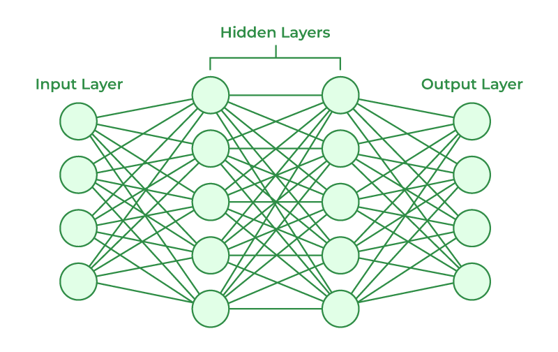
For each layer:
- Inputs to the layer:
X_i—> size B×C (activations from previous layer, on a batch size B) - Output gradients of the layer:
ΔY_i—> size B×R (gradient of loss w.r.t. outputs of this layer) - You can compute this when you backpropagate using
ΔY_i=∂L/∂Z_i - You get, for each example in the batch, a
1 × Rvector of gradients w.r.t. the outputs of this layer.
Now you can compute the gradient of the weights of each layer with:
Gi=ΔY_i^⊤Xi
which is a (R×B)⋅(B×C)=R×C matrix.
If you look at the Fisher block corresponding to layer i, it’s :
Fi≈E[(vec(Gi))(vec(Gi))^⊤]
- vec(G_i) means: take the matrix G_i “flatten” it into a vector by stacking its columns (or rows into a single long vector.
But that F_i is still a (RC×1)⋅(1×RC)=RC×RC, which is already large if R and C are large.
In the KFAC approximation we approximate F_i as the Kronecker product of two much smaller matrices:
Fi≈Ri⊗Ci
Here:
- Ri: summarizes correlations along rows (output space) of Wi.
- Ci: summarizes correlations along columns (input space) of Wi.
We trust that this aproximation works here, to learn more about KFAC:
KFAC explainedfdangel.comWhy do we do this? Because directly storing the full Fisher matrix is too expensive, but approximating it as Ri ⊗ Ci drastically reduces the memory/computation cost.
Here ⊗ is the Kronecker product:
- If A is m×m and B is n×n, then A ⊗ B is mn×mn.
Why is this useful?
Instead of inverting a huge F_I of size RC×RC, you invert bar R_i and bar C_i separately:
F_i⁻¹≈R_i^−1⊗C_i⁻¹
How does this connect to KPOP?
KPOP builds on KFAC:
- KPOP computes
bar R_iandbar C_ias in KFAC. - Then it further diagonalizes
bar R_iandbar C_iby computing their eigenvalues and eigenvectors → this is the Kronecker-Factored Eigenbasis (KFE). - KPOP rotates the gradient into this eigenbasis and runs Adam there → better conditioning, adaptive steps.
So matrices bar R_i and bar C_i can still be quite large, so we further reduce them to make optimization even easier by diagonalizing them.
Diagonalizing a matrix means:
- Finding its eigenvectors and eigenvalues.
- Rotating the matrix into the basis defined by its eigenvectors.
For a symmetric matrix M, you can write:
M=QΛQ^⊤
where:
- Q: matrix of eigenvectors
- Λ: diagonal matrix of eigenvalues
In a diagonal matrix, all the off-diagonal correlations are gone.
In out case it makes optimization much simpler & more stable, because the curvature in each direction is now uncoupled.
Meaning that:
- In standard basis: changing weight 1 affects weight 2 → messy.
- In eigenbasis: each direction is independent → you can scale & adapt each direction independently.
Think of skiing down a mountain:
- Without diagonalization: you don’t know the slope directions → you keep sliding sideways & adjusting, it is slow & unstable.
- With diagonalization: you align your skis along the steepest descent, you co faster and with more control
Quick recap:
- From Fisher → KFAC → diagonalization → so you can rescale gradients along independent, curvature-aligned directions instead of blindly following the raw gradient.
What is an EMA (Exponential Moving Average)?
Instead of using just the most recent Ri and Ci, we maintain a smoothed running average:
bar R_i←α⋅bar R_i+(1−α)⋅Ri bar C_i←α⋅bar C_i+(1−α)⋅Ci
This gives more weight to recent values, but also retains information from earlier iterations — more stable.
Now we have the ingredients to take a look at the pseudo- code
Step-by-step pseudocode
Initialization
- Parameters: θ (all weights & biases)
- Learning rate: η
- Decay rates: ααα (for KFAC EMA), β1, β2 (for Adam moments)
- Small constant: ϵ (numerical stability)
For each layer i:
- Initialize first moment estimate
m_i = 0 - Initialize second moment estimate
v_i = 0 - Initialize KFAC factors
bar R_i, bar C_ito identity or zeros
m and v are used by the Adam optimiser, it keeps track of two moving averages of the gradient, to make the optimization more stable and adaptive.
These are called:
- m: the first moment estimate → running average of the gradient itself.
- v: the second moment estimate → running average of the square of the gradient (element-wise).
Loop over training iterations:
For each iteration t:
For each weight matrix Wi in θ:
Compute gradients of weights:
- Forward & backward pass → get:
G_i=∇W_i*L→ gradient of weights Wi (R×C)X_i: activations at this layer (B×C)ΔY_i = ∇_Z_iL=: gradients of loss wrt outputs of this layer (B×R)
Update KFAC factors (EMA of covariances):
- Batch estimates of covariance:
Ci_= 1/B X_i^T X_ i quad (C×C)R_i=1/B ΔY_i^T ΔY_i quad(R×R)- Exponential moving averages (to smooth over time):
bar C_i←α bar C_i+(1−α)C_ibar R_i←α bar R_i+(1−α)Ri
(Periodically) Diagonalize KFAC factors:
- Every few iterations (e.g., t<10t or tmod 100=0):
- AllReduce: sync
bar R_iandbar C_iacross devices (if distributed) - Compute eigen-decompositions: bar C_i=Q_CΛ_CQ_C^T
bar R_i=Q_RΛ_RQ_R^T
Rotate gradient into eigenbasis (KFE):
- Transform
G_iKFE:
G_ì'=Q_R^TG_iQ_C
Now Gi′ is the gradient expressed in independent (uncorrelated) directions.
Run Adam in the KFE
For the vectorized rotated gradient Gi′G'_iGi′:
- Update first moment:
m_i leftarrow beta₁ m_i + (1 - beta₁) extvec(G'_i)
- Update second moment:
v_i leftarrow beta₂ v_i + (1 - beta₂) big( extvec(G'_i) big)²
- Bias correction:
hatm_i = (m_i)/(1 - beta₁^t), quad hatv_i = (v_i)/(1 - beta₂^t)
- Compute update in KFE:
Delta W'_i = -eta · extmat left( frachatm_isqrthatv_i + epsilon right)
Rotate update back to original space
- Transform
ΔW_i'back:
Delta W_i = Q_R Delta W'_i Q_C^ op
- Update weights:
W_i leftarrow W_i + Delta W_i
What happens in KPOP:
KPOP does not directly multiply the gradient by F⁻¹ to regularize it, like natural gradient does.
Instead:
- It takes the same intuition: "the directions of the gradient should be scaled according to the curvature in each direction".
- But it implements this idea differently:
- It approximates the Fisher using KFAC
- Then further diagonalizes R and C, i.e., moves to the Kronecker-Factored Eigenbasis (KFE).
- In this rotated basis, the curvature is already diagonalized → directions are uncorrelated.
Then instead of explicitly applying F⁻¹. it runs Adam in this eigenbasis:
update in KFE: Δθ'=−η⋅Adam(g′) . where g′ is the gradient rotated into the eigenbasis.
Instead of computing F⁻¹ KPOP finds a coordinate system where F is already diagonal (eigenbasis), and in that basis applies a smarter optimizer (Adam), which already rescales each direction properly.
Code Implementation
import torch
from torch import Tensor
from typing import List, Dict

class KPOP:
    def __init__(
        self,
        params: List[torch.nn.Parameter],
        lr: float = 1e-3,
        alpha: float = 0.95,
        beta1: float = 0.9,
        beta2: float = 0.999,
        eps: float = 1e-8
    ) -> None:
        """
        params: list of weight matrices to optimize
        lr: learning rate
        alpha: decay rate for KFAC factor EMA
        beta1, beta2: Adam parameters
        eps: numerical stability
        """
        self.params: List[torch.nn.Parameter] = params
        self.lr: float = lr
        self.alpha: float = alpha
        self.beta1: float = beta1
        self.beta2: float = beta2
        self.eps: float = eps

        # Per-parameter state
        self.state: Dict[torch.nn.Parameter, Dict] = {}
        for p in self.params:
            R, C = p.shape
            self.state[p] = {
                'm': torch.zeros_like(p),       # Adam 1st moment
                'v': torch.zeros_like(p),       # Adam 2nd moment
                'R': torch.eye(R),              # Row KFAC factor
                'C': torch.eye(C),              # Column KFAC factor
                'QR': torch.eye(R),             # Eigenvectors of R
                'QC': torch.eye(C),             # Eigenvectors of C
                'Lambda_R': torch.ones(R),     # Eigenvalues of R
                'Lambda_C': torch.ones(C),     # Eigenvalues of C
                'step': 0                       # step counter
            }

    def step(
        self,
        grads: List[Tensor],
        activations: List[Tensor],
        output_grads: List[Tensor]
    ) -> None:
        """
        grads: list of gradients ∇W (R×C)
        activations: list of X inputs (B×C)
        output_grads: list of ΔY (B×R)
        """
        for p, g, X, dY in zip(self.params, grads, activations, output_grads):
            s: Dict = self.state[p]
            R, C = p.shape
            B: int = X.shape[0]
            s['step'] += 1

            # ---- Step 1: update KFAC factors ----
            C_batch: Tensor = (X.T @ X) / B          # C × C
            R_batch: Tensor = (dY.T @ dY) / B        # R × R
            s['C'] = self.alpha * s['C'] + (1 - self.alpha) * C_batch
            s['R'] = self.alpha * s['R'] + (1 - self.alpha) * R_batch

            # ---- Step 2: diagonalize periodically ----
            if s['step'] <= 10 or s['step'] % 100 == 0:
                s['Lambda_C'], s['QC'] = torch.linalg.eigh(s['C'])  # C × C
                s['Lambda_R'], s['QR'] = torch.linalg.eigh(s['R'])  # R × R

            # ---- Step 3: rotate gradient into KFE ----
            G_kfe: Tensor = s['QR'].T @ g @ s['QC']  # R × C

            # ---- Step 4: Adam in KFE ----
            g_vec: Tensor = G_kfe.flatten()
            m: Tensor = s['m'].flatten()
            v: Tensor = s['v'].flatten()
            m = self.beta1 * m + (1 - self.beta1) * g_vec
            v = self.beta2 * v + (1 - self.beta2) * (g_vec ** 2)
            m_hat: Tensor = m / (1 - self.beta1 ** s['step'])
            v_hat: Tensor = v / (1 - self.beta2 ** s['step'])
            delta_kfe_vec: Tensor = -self.lr * (m_hat / (v_hat.sqrt() + self.eps))

            # ---- Step 5: rotate back ----
            delta_kfe: Tensor = delta_kfe_vec.view_as(G_kfe)
            delta: Tensor = s['QR'] @ delta_kfe @ s['QC'].T

            # ---- Step 6: update parameters ----
            p.data += delta

            # Save moments back
            s['m'] = m.view_as(p)
            s['v'] = v.view_as(p)
import torch.nn as nn
from torch import Tensor

B: int = 32     # batch size
C: int = 10     # input dim
R: int = 5      # output dim
num_steps: int = 500

torch.manual_seed(42)

X_data: Tensor = torch.randn(B, C)
true_W: Tensor = torch.randn(R, C)
true_b: Tensor = torch.randn(R)
Y_target: Tensor = X_data @ true_W.T + true_b

W: nn.Parameter = nn.Parameter(torch.randn(R, C))
b: nn.Parameter = nn.Parameter(torch.zeros(R))

kpop: KPOP = KPOP(params=[W], lr=1e-2)

for step in range(1, num_steps + 1):
    Y_pred: Tensor = X_data @ W.T + b
    loss: Tensor = ((Y_pred - Y_target) ** 2).mean()

    loss.backward()

    grad_W: Tensor = W.grad.clone()
    grad_b: Tensor = b.grad.clone()

    with torch.no_grad():
        dY: Tensor = 2 * (Y_pred - Y_target) / B  # B×R

        W.grad.zero_()
        b.grad.zero_()

        kpop.step(grads=[grad_W], activations=[X_data], output_grads=[dY])

        b -= 1e-2 * grad_b

    if step % 50 == 0:
        print(f"Step {step}, Loss: {loss.item():.4f}")
Pros and Cons of KPOP
Memory overhead
KPOP explicitly keeps and updates the following for each later,
bar R_i→ the row-wise Kronecker factor (size R×R)bar C_i→ the column-wise Kronecker factor (size C×C)bar Q_R, Λ_R→ eigenvectors and eigenvalues ofbar R_ibar Q_C, Λ_C→ eigenvectors and eigenvalues ofbar C_im_i,v_i→ Adam’s first and second moments (both of size R×C)
which makes the memory requirements pro portional to O(R²+C²+RC).
- The
R²andC²terms come from the KFAC/KFE factors. - The RC term comes from storing m and v, same as Adam.
In contrast:
- Adam (or AdamW) only keeps m and v (both R×C) so its memory is proportional to
O(RC)
So KPOP consumes more memory because it tracks the curvature approximation
FLOPs per progress
On the other hand, KPOP is more efficient per FLOP, because:
- The updates in the eigenbasis are better aligned with the true curvature.
- AdamW (or vanilla SGD) may require many more steps (and thus more FLOPs) to converge, because it ignores curvature and might oscillate in steep directions.
- KPOP effectively takes better, more informed steps, needing fewer of them to reach good solutions.
Empirically, this is why wall-clock time and step count to reach a target loss are lower for KPOP than Adam, despite higher cost per step.
This means:
- On H100, memory is scarce → you can’t afford big R,CR, CR,C matrices.
- On M3 Ultra, memory is abundant → you can afford large R,CR, CR,C, and you want to minimize FLOPs.
############################################################
# Explaining KPOP: Smarter Optimization with Curvature and Eigenvectors

*For Curious Readers*

## Introduction: Smarter Steps for Training Large Models

When training a machine learning model, we want to find the parameters $\	heta$ that minimize the loss $L(\	heta)$.
We adjust $\	heta$ step by step using the gradient:

$$\
abla_\	heta L = \\frac{\\partial L}{\\partial \	heta}$$

and update:

$$\	heta \\gets \	heta - \\eta \
abla_\	heta L$$

where $\\eta$ is the learning rate.

This is called **gradient descent**.
It works well, but it assumes the loss surface is smooth and equally steep in all directions — which is rarely true.
In reality, the loss surface is like a bumpy, twisted valley: steep in some directions, flat in others.
Just following the gradient leads to inefficient, zig-zagging paths.

## Why Curvature Matters

To move more effectively, we need to understand the *curvature* of the surface — how steep or flat it is in different directions.
This allows us to take big steps in flat directions and small steps in steep ones.

**Think of it like driving:** If you're on a straight highway, you can floor the accelerator. But if you're navigating hairpin turns on a mountain road, you need to slow down in sharp curves and speed up on straightaways. The "curvature" tells you when to accelerate and when to brake.

In optimization, this curvature is mathematically described by the **Hessian matrix** — the matrix of second derivatives. But computing the Hessian directly is prohibitively expensive for large neural networks.

Instead, we use the **Fisher Information Matrix**, which approximates the Hessian under certain assumptions:

$$F = \\mathbb{E} \\big[ (\
abla_\	heta \\log p(x; \	heta)) (\
abla_\	heta \\log p(x; \	heta))^\	op \\big]$$

**Why does this work?** The Fisher Information Matrix captures how much the model's predictions change when we slightly adjust the parameters. When predictions are sensitive to parameter changes (high curvature), the Fisher matrix has large values. When predictions are stable (low curvature), the Fisher matrix has small values.

The ideal update would adjust the gradient by the inverse of $F$, called the **natural gradient**:

$$\\Delta \	heta = - \\eta F^{-1} \
abla_\	heta L$$

But $F$ is huge and inverting it directly is impractical.

## The KFAC Approximation

The first clever idea is to approximate $F$ efficiently using **Kronecker-Factored Approximate Curvature** (KFAC).
It assumes some independence between layers of the model and approximates $F$ for each layer as a Kronecker product:

$$F_i \\approx R_i \\otimes C_i$$

where:

- $C_i$ is the empirical **covariance matrix of the input activations** to layer $i$:
  it captures how different input features (the entries of the input vector $x^{(i)}$) vary together across the batch.
  It is computed as:

  $$C_i = \\frac{1}{B} \\sum_{b=1}^B (x_b^{(i)} - \\mu_i)(x_b^{(i)} - \\mu_i)^\	op$$

  where $x_b^{(i)}$ is the input activation vector to layer $i$ for sample $b$, and $\\mu_i = \\frac{1}{B} \\sum_{b=1}^B x_b^{(i)}$ is the sample mean.
  In practice, the mean term is often omitted when activations are approximately zero-centered (e.g., due to batch normalization).

  Note that $x_b^{(i)}$ represents different things depending on the layer:
  - For the first layer: the actual input features (pixels, tokens, etc.)
  - For intermediate layers: the output activations from layer $i-1$

  If two input features tend to increase and decrease together in the data, $C_i$ reflects this by having a large positive off-diagonal entry.
  If they are independent, the corresponding entry is close to zero.

- $R_i$ is the empirical **covariance matrix of the output gradients** (errors) at layer $i$:
  it captures how the components of the error signal (the gradient of the loss with respect to the layer's outputs) vary together across the batch.
  It is computed as:

  $$R_i = \\frac{1}{B} \\sum_{b=1}^B (y_b^{(i)} - \
u_i)(y_b^{(i)} - \
u_i)^\	op$$

  where $y_b^{(i)}$ is the output gradient vector (error signal) at layer $i$ for sample $b$, and $\
u_i = \\frac{1}{B} \\sum_{b=1}^B y_b^{(i)}$ is the sample mean.
  In practice, the mean term is often omitted when gradients are approximately zero-centered.

  Note that $y_b^{(i)}$ represents the gradients of the loss with respect to the outputs of layer $i$:
  - These are the error signals flowing backward through the network
  - They indicate how much each output dimension contributes to the total loss

  If two output gradients tend to rise or fall together (meaning errors at two outputs are correlated), $R_i$ reflects this correlation.

Why compute these covariances?
The optimizer aims to approximate the curvature of the loss surface with respect to the weights $W_i$.
The exact curvature involves the second derivative of the loss — or equivalently, the Fisher Information Matrix — which is expensive to compute.
However, under some assumptions, the Fisher block for $W_i$ can be approximated by the Kronecker product $R_i \\otimes C_i$.
Thus, $R_i$ and $C_i$ summarize how the input signals and output errors co-vary, providing an efficient approximation to curvature.

**But there's still a problem:** Even though KFAC makes the Fisher matrix easier to compute, $R_i$ and $C_i$ are still full matrices with off-diagonal entries. This means different gradient directions are still coupled together, making optimization complex.

**The KPOP insight:** What if we could find a coordinate system where the curvature matrix becomes diagonal? In such a system, each direction would be completely independent, and we could optimize each one separately. This is exactly what eigendecomposition achieves!

## Updating Kronecker Factors During Training

So far we've explained how to compute $R_i$ and $C_i$, but there's a crucial implementation detail: these matrices need to be updated continuously during training to track the changing curvature.

KPOP uses **Exponential Moving Averages (EMA)** to adapt the Fisher information matrix as training progresses. Here's how it works:

**Step 1: Compute batch-level estimates**
At each training iteration, compute fresh estimates from the current batch:

$$C_i^{(t)} = \\frac{1}{B} X_i X_i^\	op \\quad \	ext{and} \\quad R_i^{(t)} = \\frac{1}{B} \\Delta Y_i \\Delta Y_i^\	op$$

where:
- $X_i \\in \\mathbb{R}^{C \	imes B}$ is the activation matrix for layer $i$
- $\\Delta Y_i \\in \\mathbb{R}^{R \	imes B}$ is the gradient matrix (error signals) for layer $i$
- $B$ is the batch size
- $t$ denotes the current training iteration

**Step 2: Update EMA estimates**
Instead of using the raw batch estimates, maintain running averages:

$$\	ilde{C}_i^{(t)} \\leftarrow \\alpha \	ilde{C}_i^{(t-1)} + (1-\\alpha) C_i^{(t)}$$

$$\	ilde{R}_i^{(t)} \\leftarrow \\alpha \	ilde{R}_i^{(t-1)} + (1-\\alpha) R_i^{(t)}$$

where $\\alpha \\in [0,1)$ is the decay parameter (typically $\\alpha = 0.95$ or $\\alpha = 0.99$).

**Why use EMA instead of raw batch estimates?**
- **Stability**: Raw batch estimates are noisy; EMA provides smooth, stable curvature estimates
- **Memory of past geometry**: The curvature information from previous iterations helps guide current updates
- **Robustness**: Reduces sensitivity to outlier batches or sudden changes in data distribution

**The eigendecomposition step:**
The eigenvectors and eigenvalues are computed from the EMA estimates $\	ilde{R}_i$ and $\	ilde{C}_i$, not the raw batch estimates:

$$\	ilde{R}_i = Q_R \\Lambda_R Q_R^\	op, \\quad \	ilde{C}_i = Q_C \\Lambda_C Q_C^\	op$$

This EMA mechanism is what makes KPOP practical for real training scenarios!

## Why Eigenvectors and Eigenvalues Help

Even with KFAC, $R_i$ and $C_i$ are still full matrices — so different directions of the gradient still interact.
To make each direction independent, we diagonalize $R_i$ and $C_i$ by computing their **eigenvalues** and **eigenvectors**:

$$R_i = Q_R \\Lambda_R Q_R^\	op, \\quad C_i = Q_C \\Lambda_C Q_C^\	op$$

where:
- $Q_R$, $Q_C$ are matrices whose columns are eigenvectors — special directions in which the matrix acts by scaling only.
- $\\Lambda_R$, $\\Lambda_C$ are diagonal matrices of eigenvalues — the amount of scaling in each eigenvector direction.

**Why is this crucial?** Think of it this way: if you're hiking in mountains, you want to know which directions are steep cliffs (high eigenvalues) versus gentle slopes (low eigenvalues). The eigenvectors point you toward these natural directions of the landscape, while eigenvalues tell you how steep each direction is.

In this eigenbasis, the curvature becomes diagonal — each direction is independent and we know exactly how steep it is (from the eigenvalues). This transforms a complex, intertwined optimization problem into a collection of simple, independent 1D problems.

## Transforming the Gradient

Here is the core idea of KPOP:

1. Compute the gradient of the loss with respect to the weights at layer $i$, denoted $G_i$.

2. Rotate $G_i$ into the eigenbasis:

   $$G'_i = Q_R^\	op G_i Q_C$$

   This expresses the gradient in terms of the eigenvectors of $R_i$ and $C_i$.

   In this rotated space:
   - The curvature is diagonal.
   - Each direction (each entry in $G'_i$) corresponds to an independent direction of steepest descent.

3. Apply an adaptive optimizer (like Adam) to $G'_i$, adjusting the step in each direction according to its eigenvalue and past gradients:

   $$m_t = \\beta_1 m_{t-1} + (1-\\beta_1) G'_i$$

   $$v_t = \\beta_2 v_{t-1} + (1-\\beta_2) (G'_i)^2$$

   $$\\hat{m}_t = \\frac{m_t}{1-\\beta_1^t}, \\quad \\hat{v}_t = \\frac{v_t}{1-\\beta_2^t}$$

   The standard Adam update is then applied in the rotated space:

   $$\\Delta W'_i = - \\eta \\frac{\\hat{m}_t}{\\sqrt{\\hat{v}_t} + \\epsilon}$$

   **Why does this work without explicit eigenvalue preconditioning?** The eigenvalues have already done their job by rotating us into the eigenbasis where the curvature is diagonal. In this space, Adam's assumption of independent directions becomes valid, so standard Adam works optimally.

4. Rotate the update back to the original parameter space:

   $$\\Delta W_i = Q_R \\Delta W'_i Q_C^\	op$$

In short:
rotate the gradient into the eigenbasis (where directions are independent), apply Adam there, and rotate back.
This aligns the update with the curvature, leading to more efficient steps.

### Addressing Common Misconceptions

**Misconception 1: "KPOP is computationally less complex"**

This is **wrong**! KPOP is actually **MORE expensive** per step than Adam:
- Computing eigendecompositions: $O(d^3)$ for each covariance matrix
- Matrix multiplications for rotations: $O(d^2)$ operations
- Adam only needs element-wise operations: $O(d)$

**Why use KPOP then?** Because it converges in **fewer steps**. Think of it like:
- Adam: cheap car, long journey (many steps)
- KPOP: expensive car, short journey (fewer steps)

**Misconception 2: "The space is reduced to 1D"**

The space is **NOT** reduced to 1D! Here's what actually happens:

- **Before rotation**: Optimization problem is coupled (changing one parameter affects how you should change others)
- **After rotation**: Optimization becomes a collection of **independent** problems, each still in its own dimension
- We still have the same number of parameters, just in a better coordinate system

**Analogy:** Imagine you're solving a 2D maze, but the walls are diagonal. Instead of moving "northeast" and "southeast" (coupled directions), you rotate your view so you can move "north" and "east" independently. You're still in 2D, but navigation becomes much simpler.

**Misconception 3: "Only eigenvectors are used"**

Both eigenvectors AND eigenvalues are crucial:
- **Eigenvectors** ($Q_R, Q_C$): Define the rotation to independent coordinates
- **Eigenvalues** ($\\Lambda_R, \\Lambda_C$): Define the natural coordinate system where the curvature is diagonal, making Adam's assumptions valid

The eigenvalues work *implicitly* by defining the coordinate transformation, not by explicit preconditioning of step sizes.

## A Concrete Example: Understanding the Rotation

Let's work through a simple $2\	imes 2$ example to see exactly what "rotation" means.

**Setup:** Imagine a layer with 2 inputs and 2 outputs, so the weight matrix $W$ is $2\	imes 2$:

$$W = \\begin{pmatrix} w_{11} & w_{12} \\\\ w_{21} & w_{22} \\end{pmatrix}$$

**Step 1: Compute the gradient**
Suppose our gradient is:

$$G = \\begin{pmatrix} 1.0 & 0.5 \\\\ 0.5 & 1.0 \\end{pmatrix}$$

**Step 2: Compute covariance matrices**
From our batch, suppose we get:

$$C = \\begin{pmatrix} 2.0 & 1.0 \\\\ 1.0 & 1.0 \\end{pmatrix}, \\quad R = \\begin{pmatrix} 1.5 & 0.5 \\\\ 0.5 & 0.5 \\end{pmatrix}$$

**Step 3: Find eigenvectors (the "rotation" matrices)**
For $C$:

$$C = Q_C \\Lambda_C Q_C^\	op = \\begin{pmatrix} 0.85 & -0.53 \\\\ 0.53 & 0.85 \\end{pmatrix} \\begin{pmatrix} 2.62 & 0 \\\\ 0 & 0.38 \\end{pmatrix} \\begin{pmatrix} 0.85 & 0.53 \\\\ -0.53 & 0.85 \\end{pmatrix}$$

For $R$:

$$R = Q_R \\Lambda_R Q_R^\	op = \\begin{pmatrix} 0.92 & -0.39 \\\\ 0.39 & 0.92 \\end{pmatrix} \\begin{pmatrix} 1.82 & 0 \\\\ 0 & 0.18 \\end{pmatrix} \\begin{pmatrix} 0.92 & 0.39 \\\\ -0.39 & 0.92 \\end{pmatrix}$$

**Step 4: "Rotate" the gradient**

$$G' = Q_R^\	op G Q_C = \\begin{pmatrix} 0.92 & 0.39 \\\\ -0.39 & 0.92 \\end{pmatrix} \\begin{pmatrix} 1.0 & 0.5 \\\\ 0.5 & 1.0 \\end{pmatrix} \\begin{pmatrix} 0.85 & -0.53 \\\\ 0.53 & 0.85 \\end{pmatrix}$$

$$G' = \\begin{pmatrix} 1.31 & 0.02 \\\\ 0.02 & 0.69 \\end{pmatrix}$$

**What happened?**
- **Original gradient $G$**: Had off-diagonal terms (0.5), meaning the gradient directions were coupled
- **Rotated gradient $G'$**: Nearly diagonal! The off-diagonal terms (0.02) are almost zero

**Why is this powerful?**
In the original coordinates, updating $w_{11}$ affects the loss in a way that depends on $w_{12}$, $w_{21}$, and $w_{22}$. Everything is tangled together.

In the rotated coordinates, each direction is nearly independent. We can optimize each direction separately without worrying about complex interactions.

**Step 5: Apply Adam in the rotated space**
Now we simply apply Adam to $G'$ where directions are independent:

$$\	ext{Adam\\_output} = \\begin{pmatrix} -0.131 & -0.002 \\\\ -0.002 & -0.069 \\end{pmatrix}$$

**Why is this effective without explicit eigenvalue scaling?**

The magic happens because we're now in the eigenbasis! The eigenvalues have already "rotated" us into a coordinate system where:
- Each direction is independent (nearly diagonal gradient)
- Adam's assumptions are valid
- The curvature information is implicitly encoded in the coordinate system itself

**Step 6: Rotate back**

$$\\Delta W = Q_R (\	ext{Adam\\_output}) Q_C^\	op$$

**What did we accomplish?**

1. **Found natural coordinates**: The eigenvectors revealed the coordinate system where optimization directions are independent
2. **Identified steepness**: The eigenvalues told us which directions are steep (high curvature) vs flat (low curvature)
3. **Smart step sizing**: We took small steps in steep directions, big steps in flat directions
4. **No more zig-zagging**: Instead of fighting against the problem's geometry, we aligned with it

**The key insight:** KPOP doesn't reduce complexity - it **transforms** the problem into a form where each direction can be optimized independently with appropriate step sizes. This leads to faster convergence despite higher per-step cost.

**Visual analogy:** Imagine you're trying to navigate in a city, but the streets are at weird angles. Instead of giving directions like "go 3.2 blocks at 23° angle," you:
1. Rotate your map so the streets align with horizontal/vertical
2. Give simple directions: "go 2 blocks north, 4 blocks east"
3. Rotate back to the original map orientation

That's exactly what KPOP does with gradients!

## Why Combine with Adam?

Adam already adapts learning rates for each parameter based on past gradients, but it assumes the curvature is already diagonal — which is not true in the original space.
By moving into the eigenbasis where curvature is diagonal, this assumption becomes true, making Adam more effective.

## Pros and Cons of KPOP

### Memory Overhead

KPOP explicitly keeps and updates, for each layer $i$:
- $R_i$ — output gradient covariance matrix ($d_{out}^{(i)} \	imes d_{out}^{(i)}$)
- $C_i$ — input activation covariance matrix ($d_{in}^{(i)} \	imes d_{in}^{(i)}$)
- $Q_{R,i}, \\Lambda_{R,i}$ — eigenvectors and eigenvalues of $R_i$
- $Q_{C,i}, \\Lambda_{C,i}$ — eigenvectors and eigenvalues of $C_i$
- $m_i, v_i$ — Adam's first and second moments ($d_{out}^{(i)} \	imes d_{in}^{(i)}$)

where $d_{out}^{(i)}$ and $d_{in}^{(i)}$ are the output and input dimensions of layer $i$, respectively.

This makes the memory requirement per layer:

$$O\\big((d_{out}^{(i)})^2 + (d_{in}^{(i)})^2 + d_{out}^{(i)} \\cdot d_{in}^{(i)}\\big)$$

By contrast, Adam only keeps $m$ and $v$ ($d_{out}^{(i)} \	imes d_{in}^{(i)}$) → $O(d_{out}^{(i)} \\cdot d_{in}^{(i)})$.

So KPOP consumes more memory because it tracks the curvature approximation.

### FLOPs per Progress

On the other hand, KPOP is more efficient per FLOP because:
- The updates in the eigenbasis are better aligned with the true curvature.
- Adam or SGD may require many more steps (and thus more FLOPs) to converge because they ignore curvature and may oscillate.
- KPOP takes more informed steps, needing fewer of them to reach a good solution.

Empirically, wall-clock time and step count to reach a target loss are lower for KPOP than Adam, despite higher cost per step.

### Hardware Considerations

This trade-off depends on hardware:
- On NVIDIA H100, memory is scarce — so the $(d_{out}^{(i)})^2 + (d_{in}^{(i)})^2$ terms are expensive.
- On Apple M3 Ultra, memory is abundant — so you can afford the extra curvature matrices and benefit from fewer FLOPs.

**Concrete example:** Consider a transformer layer with $d_{in} = d_{out} = 4096$.
- **Adam memory:** $2 \	imes 4096^2 \\approx 32M$ parameters (for $m$ and $v$)
- **KPOP memory:** $32M + 2 \	imes 4096^2 \\approx 64M$ parameters (Adam + curvature matrices)

**On H100 (80GB HBM):** Training a 70B parameter model is already tight on memory. The extra 32M parameters per layer $\	imes$ 100 layers = 3.2B extra parameters might not fit.

**On M3 Ultra (192GB unified memory):** The extra memory is easily affordable, and KPOP's faster convergence (requiring 30–50% fewer steps) often leads to better wall-clock time despite higher per-step cost.

**The sweet spot:** KPOP shines when memory is available but compute time is the bottleneck — making it ideal for research settings, fine-tuning, or training on high-memory consumer hardware.

## Conclusion

KPOP is an elegant optimizer that:
- Learns the curvature of the loss landscape.
- Rotates into the natural axes of that landscape (eigenbasis).
- Applies adaptive updates (like Adam) efficiently in that space.
- Rotates back to the original parameters.

This allows it to move straight toward the minimum instead of zig-zagging — leading to faster, more robust training, even on consumer-grade hardware.

**When should you use KPOP?**
- You have sufficient memory (at least 2× what Adam needs)
- Training time is more important than memory efficiency
- You're training on consumer hardware with abundant memory
- You need robust convergence on complex loss landscapes

**When to stick with Adam:**
- Memory is extremely constrained (e.g., edge devices, large-scale distributed training)
- Your model already converges quickly with simple optimizers
- You're optimizing for minimal memory footprint over training speed

**The big picture:** KPOP represents a fundamental shift from "one-size-fits-all" optimizers toward "geometry-aware" optimization. By understanding and adapting to the shape of the loss landscape, it achieves what mathematicians call "quadratic convergence" — the holy grail of optimization where each step becomes exponentially more effective.

As neural networks grow larger and more complex, this type of curvature-aware optimization may become essential for training the next generation of AI models efficiently.

**Key ideas:**
- Fisher matrix captures curvature.
- KFAC approximates Fisher efficiently.
- Eigenvectors/eigenvalues align us with independent directions.
- Adam adapts step size for each direction.

Together, they make KPOP a powerful optimizer for large-scale training.

## Further Reading

If you want to explore further:
- Martens & Grosse (2015): KFAC
- Kingma & Ba (2015): Adam
- George et al. (2018): Kronecker-Factored Eigenbasis